A Simple Way to Check Bearing Capacity of Foundations Adjacent to Slopes

Shallow foundations are often placed close to slopes, excavations, road cuts, quay walls, or terrain breaks. In these situations, the bearing capacity can be significantly lower than the value calculated for the same foundation on flat terrain. The reason is physical: the failure mechanism on the slope side is not fully confined by soil. The passive resistance is reduced, and the foundation may reach failure at a lower vertical load.

This was the motivation for the method I developed. The aim was not to replace finite-element analysis, finite-element limit analysis, or detailed slope-stability calculations. The aim was to provide a simplified, transparent, mechanism-based check for shallow strip foundations located adjacent to slopes.

In routine design, the first question is often simple: is the foundation sufficiently far from the slope crest, or does the slope still reduce the bearing capacity? The method answers this by connecting two familiar limiting cases:

the foundation at the slope crest;
the foundation on flat terrain.

Between these two cases, the influence of the slope reduces as the setback distance increases.

The approach in brief

Consider a strip foundation of width placed at a setback distance from the crest of a slope with inclination β. At the crest, the slope has its maximum influence. At a sufficiently large setback, the failure mechanism no longer reaches the slope and the flat-ground solution is recovered.

The method represents this transition using a modified slope angle β’.

At the crest,

At the no-influence setback distance,

Thus, the calculation does not switch abruptly from a slope case to a flat-ground case. Instead, the mechanism changes progressively as the foundation is moved away from the crest.

Drained case: mechanism and envelope

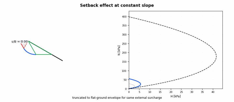
Figure 1 shows the drained case. The slope angle is kept constant while the setback distance is increased. The left side shows the change in the failure mechanism. The right side shows the corresponding – interaction envelope.

Figure 1. Drained failure mechanism and H-N envelope as setback increases. The slope angle is constant and the setback wedge unit weight is taken equal to the soil unit weight.

Near the slope crest, the failure mechanism is strongly influenced by the slope. As the setback increases, the influence of the slope decreases. Eventually, the mechanism approaches the flat-ground case.

For drained conditions, the method is expressed using the effective stress parameters c’, and φ’. The assumed mechanism consists of an active Rankine zone, a transition zone and a passive Rankine zone. The transition zone is a logarithmic spiral, as expected for a frictional bearing-capacity mechanism.

A useful way to write the drained formulation is to use the attraction term

A peculiarity of the drained case is that the no-influence setback distance is not only a geometric quantity. It depends on the foundation width, the friction angle and the mobilized roughness.

Another peculiarity is the contribution from unit weight. Near the crest, the passive side of the mechanism is restricted, and the contribution can be significantly reduced. As the foundation is moved away from the crest, the passive mechanism becomes more complete and the capacity approaches the flat-ground value.

The implementation may also include a setback wedge surcharge. In the demonstration above, the setback wedge unit weight is taken equal to the soil unit weight:

This surcharge can increase the calculated resistance. For design use, however, it is usually sensible to prevent the slope-adjacent capacity from exceeding the corresponding flat-ground capacity for the same surcharge condition.

Undrained case

For undrained conditions, the method is expressed using the undrained shear strength, c_u. The undrained case can be viewed as the limiting case of the drained mechanism when the friction angle is zero:

The logarithmic spiral transition zone then becomes a circular arc. The undrained mechanism is therefore geometrically simpler than the drained one.

The vertical bearing resistance can be written conceptually as

where is the applied surcharge term and is the undrained bearing-capacity factor associated with the mechanism.

A peculiarity of the undrained interaction problem is that the horizontal resistance is directly linked to the mobilized undrained strength:

Here, is the mobilized roughness ratio and cu,mob is the mobilized undrained shear strength. This makes the undrained – envelope easier to interpret than the drained one. The horizontal component is controlled directly by r, while the vertical component is controlled by Nc, surcharge and the changing mechanism geometry.

The undrained formulation does not contain a drained-type N_gamma contribution. Soil unit weight does not enter the undrained bearing-capacity expression in the same way as in the drained formulation. However, a setback wedge surcharge may still be included as an external stabilizing surcharge where appropriate.

How to implement the mechanism-based method

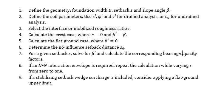
A practical implementation can be organized as follows.

The optional flat-ground upper limit can be written as

This prevents the bearing capacity adjacent to the slope from exceeding the equivalent flat-ground value.

Linear interpolation simplification

A simpler approximation is to interpolate linearly between the crest case and the flat-ground case. This simplification was first mentioned in Døssland’s (1980).

The idea is direct. First calculate the bearing capacity at the slope crest. Then calculate the bearing capacity for flat terrain. Finally, interpolate between these two values using the setback distance.

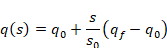
Let the bearing capacity at the slope crest be q0, the flat-ground bearing capacity be , and the no-influence setback distance be s0. For a foundation located between the crest and the no-influence distance,

for

For setback distances beyond the no-influence distance,

for

The same idea can be applied to – interaction envelopes. The interpolation is then performed point by point between the crest envelope and the flat-ground envelope:

This linear-interpolation version is attractive because it is easy to implement and explain. It is best treated as a preliminary design check or a sensitivity tool, not as a substitute for a full mechanism-based or numerical analysis.

Limitations of the method

The method is simplified and should be used with engineering judgement. It is based on an assumed failure mechanism and is most naturally suited to strip foundations under plane-strain conditions.

It does not explicitly model progressive failure, strain softening, complex layering, anisotropy, groundwater effects, cyclic degradation, or three-dimensional foundation shape effects unless these are introduced separately through engineering approximations.

The method checks bearing capacity adjacent to a slope. It does not by itself prove that the slope is globally stable. This distinction is important: a foundation may have adequate local bearing capacity while the slope as a whole may still be unsafe.

The method is also sensitive to the selected soil parameters. In drained analysis, the friction angle and effective unit weight strongly affect the result. In undrained analysis, the selected undrained shear strength profile is critical.

Always check slope stability

A bearing-capacity check adjacent to a slope should be accompanied by a slope-stability check. The local bearing-capacity mechanism and the global slope-failure mechanism are not necessarily the same.

The engineer should check whether the slope is stable before and after foundation loading. This is especially important for clay slopes, high slopes, slopes with weak layers, slopes affected by groundwater and slopes close to excavations.

If the slope stability factor of safety is low, the bearing-capacity result may not govern the design. The controlling failure mode may instead be a global or compound slope failure.

Advanced methods

For important projects, difficult ground conditions or marginal stability cases, more advanced methods should be considered. These include:

limit equilibrium slope-stability analysis;
finite-element analysis with strength reduction;
finite-difference analysis;
upper-bound and lower-bound limit analysis;
finite-element limit analysis;
numerical modelling with staged excavation and construction;
coupled consolidation analysis for soft clays;
probabilistic analysis where spatial variability of strength is important.

These methods can capture effects that are outside the simplified formulation, such as nonhomogeneous soil, groundwater, staged loading, deformation compatibility and global failure mechanisms.

Closing remarks

The bearing capacity of shallow foundations adjacent to slopes is controlled by both soil strength and geometry. The setback distance from the crest is especially important.

The method I proposed provides a simple way to account for this effect. At its most basic level, the bearing capacity can be interpolated linearly between the crest case and the flat-ground case. At a more detailed level, the method uses a changing mechanism governed by the modified slope angle .

For drained conditions, the method gives a frictional mechanism with a logarithmic spiral transition zone. For undrained conditions, the same framework reduces to a circular-arc mechanism. Both cases can be used to estimate bearing capacity and to generate – interaction envelopes.

The method is deliberately simple, visual and practical. Its purpose is to help engineers check shallow foundations adjacent to slopes while still recognizing when a full slope-stability or numerical analysis is required.

References

Tsegaye, A. B. (2019). Bearing capacity of shallow foundations that are situated at a varying distance from slopes. XVII European Conference on Soil Mechanics and Geotechnical Engineering.

Døssland, T. (1980). Forankring av støttekonstruksjo-ner med horisontale friksjonselement. NorgesTeknsike Høgskole Universitet.

Meyerhof, G. G. (1957). The ultimate bearing capacity of foundations on slopes. Proceedings of the 4th International Conference on Soil Mechanics and Foundation Engineering.

Equivalent Quasi-Static FEM Procedure for Estimating Settlement from Tipping or Dumping Impact

1. Introduction

Tipping, dumping, or accidental dropping of heavy masses can generate short-duration impact loads that produce local settlement and permanent ground deformation. Such effects may be critical where the impact occurs close to foundations, retaining walls, buried services, pavements, or other structures sensitive to ground movement.

A fully dynamic analysis of these events would require modelling contact behaviour, inertia, damping, stress-wave propagation, strain-rate effects, and the time-dependent response of the soil. For practical engineering assessment, however, an equivalent quasi-static approach may be appropriate where the primary design concern is residual settlement rather than transient vibration or peak impact force.

The proposed approach is based on an energy-balance principle. This principle is consistent with the treatment of dropped-object loading in DNV-RP-C204, where the impact is represented as a kinetic-energy problem. In that method, the impact energy is dissipated as strain energy in the impacted component and, where relevant, in the dropped object itself. The dissipated energy is evaluated from force–deformation relationships, with the absorbed energy corresponding to the area under the load–deformation curve.

In the present method, the same energy-balance concept is adapted to soil deformation. The kinetic energy of the falling or tipped mass is assumed to be converted into internal work in the soil, causing both elastic and plastic deformation. The method can be implemented in a finite element model by applying incremental loading over the assumed impact area and calculating the work done from the resulting load–deformation response.

2. Energy Basis

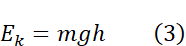
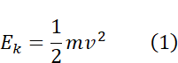
A mass m moving with velocity v at impact has kinetic energy:

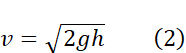
For a freely falling mass from height h, neglecting air resistance and other losses, the impact velocity is:

and therefore:

where g is gravitational acceleration.

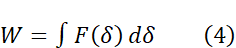
During impact, the kinetic energy is dissipated as deformation work in the soil and, where relevant, in the impacting material or intermediate layers. The work done by the impact force is:

where F(δ) is the applied force as a function of deformation δ. For elastoplastic soil, this relationship is generally nonlinear. The work is therefore calculated as the area under the load–deformation curve, not simply as force multiplied by deformation.

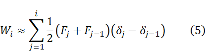
For incremental FEM results, the accumulated work may be approximated as:

where F_j and δ_j are the applied load and corresponding deformation at increment j.

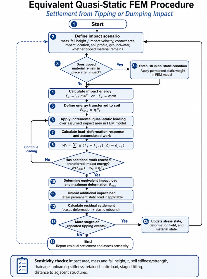
3. Proposed FEM Procedure

The following quasi-static FEM procedure may be adopted.

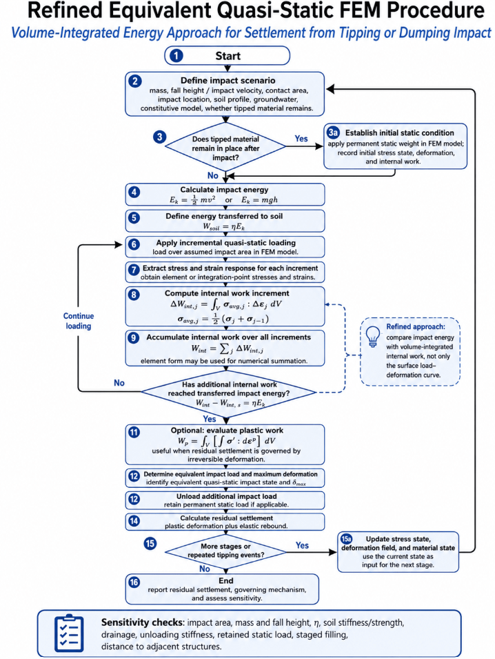
4. Extended Volume-Integrated Energy Approach

The load–deformation method evaluates external work at the load application point or over the assumed impact area. A more detailed approach is to evaluate the internal work accumulated throughout the deforming soil volume.

In a quasi-static FEM analysis, the external work calculated from the load–deformation curve and the internal work integrated over the model volume should be broadly consistent, provided that all relevant energy terms are included. However, the volume-integrated method gives additional insight into where the impact energy is dissipated. It can be used to identify whether the response is dominated by local bearing failure, deeper shear deformation, lateral spreading, or wider ground settlement.

5. Limitations

The method is approximate. It is an equivalent quasi-static approach, not as a full dynamic impact analysis. It does not explicitly model stress-wave propagation, inertia, damping, contact duration, strain-rate effects, or dynamic amplification. These effects may be important for large drop heights, stiff ground conditions, short impact durations, or sensitive nearby structures.

The result is also sensitive to the assumed contact area. In reality, the contact area may change during impact due to penetration, crushing, spreading, or rotation of the tipped material.

Soil behaviour is nonlinear and path-dependent. The calculated residual settlement depends on the soil constitutive model, drainage condition, stiffness degradation, plasticity model, and unloading stiffness. For saturated fine-grained soils, post-impact consolidation may also be relevant.

6. Recommended Sensitivity Checks

The following parameters should be varied to assess the robustness of the result:

impact area;
mass and fall height;
energy transfer factor η;
soil stiffness and strength;
drainage condition;
unloading stiffness;
static load from retained tipped material;
staged filling sequence;
distance to adjacent structures.

Where adjacent structures are sensitive to vibration or transient movement, the quasi-static analysis should be supplemented by dynamic analysis, field monitoring, or empirical vibration assessment.

7. Conclusion

The proposed method provides a practical quasi-static FEM procedure for estimating soil settlement caused by tipping or dumping impacts. It is based on the same energy-balance principle used in established dropped-object and impact-assessment methods, where kinetic energy is converted into deformation work obtained from a load–deformation curve.

The method is useful where the main design concern is residual settlement. Its main advantages are simplicity, compatibility with conventional FEM analysis, and the ability to account for site-specific geometry, soil stratigraphy, boundary conditions, and staged loading.

However, the method does not capture the full dynamic impact response. It should therefore be applied with sensitivity analyses and, where consequences are significant, calibrated or checked against field observations, trial tipping, falling-weight tests, or dynamic numerical analysis.

Eurocode 7 Design Approaches: Hidden Pitfalls and Practical Recommendations

In Eurocode 7, the partial factors used for STR/GEO limit state verification are grouped into sets for actions or effects of actions (A), soil or material parameters (M), and resistances (R). The selected combination depends on the relevant Design Approach and may also be further specified in the National Annex.

Design Approach 2 (DA2) uses the combination A1 + M1 + R2. In this approach, partial factors are applied to the actions, or to the effects of actions, and to the ground resistances. In numerical analyses, DA2 is often applied in the form commonly referred to as DA2*, where the analysis is carried out using characteristic soil parameters and unfactored or adjusted actions, and the resulting structural effects are subsequently factored to obtain design values.

Design Approach 3 (DA3) uses the combination (A1 or A2) + M2 + R3, where A1 is applied to structural actions and A2 to geotechnical actions. In this approach, partial factors are applied to the actions or effects of actions and to the ground strength parameters. For slope stability and overall stability analyses, actions acting on the soil, such as structural loads, traffic loads, and terrain loads, are generally treated as geotechnical actions.

These approaches can be illustrated by considering the design of a sheet pile wall. In DA2 or DA2*, external loads such as traffic loads or structural loads may be applied with appropriate adjustment factors. The analysis is then typically carried out using characteristic soil parameters. The resulting structural forces in the sheet pile wall and support system are subsequently factored to obtain design values.

In DA3, the relevant external loads, such as traffic loads, terrain loads, and other actions, are factored before the analysis using their respective partial factors. It is important to distinguish between structural actions and geotechnical actions, since different action factor sets may apply. The soil strength parameters, such as c′, ϕ′, or su, are also reduced according to the relevant material partial factors. For example, in an undrained analysis, the target material factor may be 1.4, or another value specified in the applicable National Annex or local code. The design values of the structural forces in the sheet pile wall and associated support systems may then be taken directly from the calculation results.

However, both approaches have practical limitations. For DA2 or DA2*, a key difficulty arises when the required safety level depends on the soil type, consequence or reliability class, or expected failure mechanism. This is relevant, for example, in Norwegian practice, where material factors for soil strength may depend on the reliability class and the type of failure mechanism.

In finite element analysis, a common DA2* procedure is to carry out the calculation with characteristic soil parameters and then apply a common factor to the resulting effects. In some cases, the applied loads may be adjusted before the analysis to account for differences between the action factors and the factor later applied to the effects. For example, if a variable load requires a factor of 1.5, but a common factor of 1.35 is later applied to the calculated effects, the variable load may first be adjusted by a factor of 1.5/1.35 before the analysis. The common factor is then applied afterwards to the calculated structural effects.

While this procedure can account for differences in action factors, it is more difficult to account for variations in the required material factor on soil strength or resistance when only one common factor, such as 1.35, is applied to the resulting effects. One possible remedy is to use consequence-class- or reliability-class-dependent factors when deriving ULS design effects from the calculated results.

This issue is less problematic in DA3, since the action factors and material factors can be incorporated directly in the numerical model. The strength parameters can be reduced to the required design values, with the required material factor depending on the applicable National Annex, consequence or reliability class, and possibly the expected failure mechanism. The resulting ULS effects may then be obtained directly from the finite element calculation.

Nevertheless, DA3 also has limitations. When structural forces are derived from a reduced-strength state close to failure, the associated displacements may become very large. This can result in significant force redistribution and unrealistically high structural effects in the sheet pile wall and support system.

For this reason, a practical approach in some cases may be to use DA3 for the verification of overall stability, while adopting DA2 or DA2* for the structural design of the wall and support members, provided this is consistent with the applicable National Annex and project requirements.

However, when DA2* is used, the applied factors should be adjusted appropriately so that the resulting design effects reflect the required safety level for the relevant consequence class or reliability class.

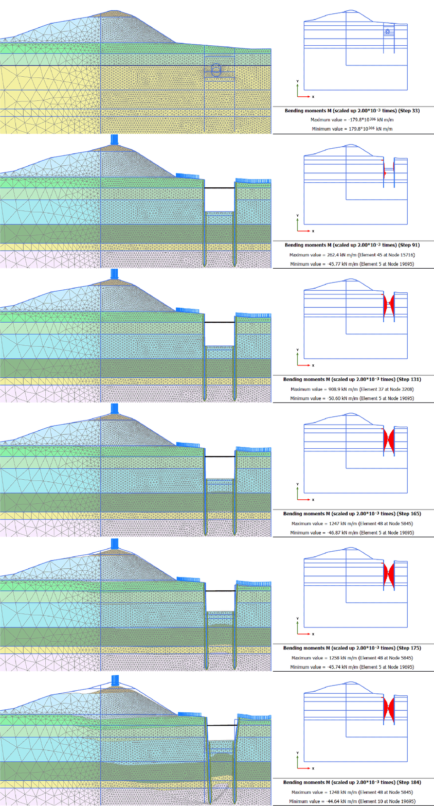
In the example below, a 2D PLAXIS analysis of a sheet-pile-wall-supported excavation adjacent to a railway is presented. The global stability is only marginally above the required safety level. The left-hand side shows the progression of mesh deformation before and during the safety analysis, while the right-hand side shows how the bending moment in the sheet pile wall increases during the same analysis stages.

An elastic plate model is used so that the increase in bending moment is not artificially capped. If an elastoplastic plate had been selected instead, the bending moment would have been limited by the axial force–bending moment interaction envelope, and the analysis would not show the potential for further moment development.

In this example, the increase in bending moment stops only because the specified number of strength reduction steps, in this case 100, has been completed. If the safety analysis had been allowed to continue for additional steps, the bending moment would likely have continued to increase.

Capacity of steel core piles – a pseudo elastic approach

Steel core piles are often regarded as the “Rolls-Royce” of foundation systems: they are highly capable, but also expensive, and their production and transportation come with a considerable carbon footprint. That alone makes optimal design not merely desirable, but necessary. Yet current practice is often far from optimal. In many cases, steel core piles are designed only for the elastic capacity of the steel core, while the contribution of the concrete infill and the steel casing is simply ignored. Structurally, this is difficult to justify. The pile is a composite member, and there is no fundamental reason why its resistance should not be assessed on that basis, particularly when corrosion losses in the casing can be accounted for explicitly, as is already done for steel pipe piles, and when the steel core can be detailed to ensure adequate interaction with the concrete.

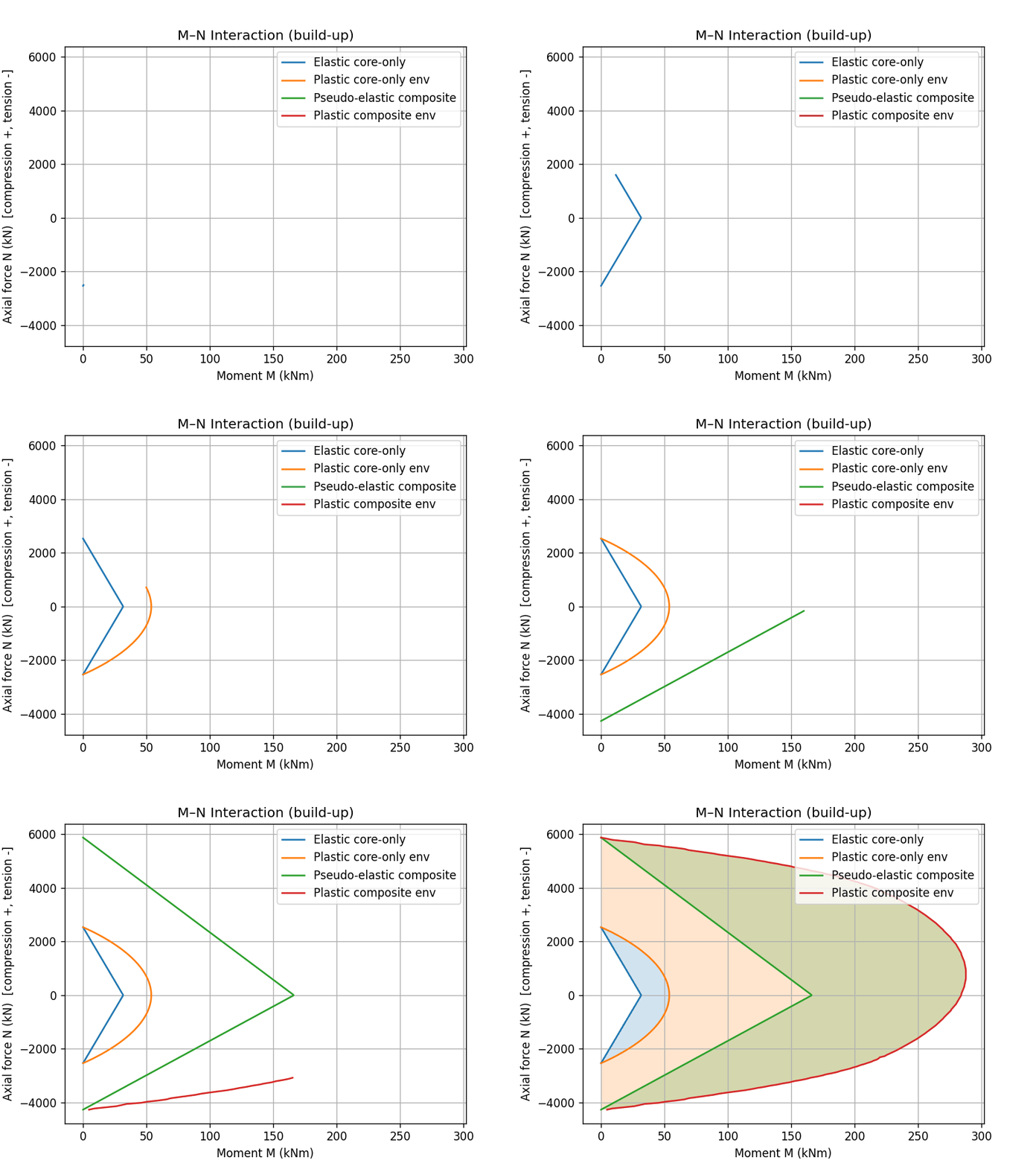
For some time, I have been reflecting on this inconsistency and about six years ago I developed a simplified method for estimating the capacity of steel core piles, which I refer to as the pseudo-elastic approach and would like to share here. The aim of the method is to provide a practical and reasonable estimate of composite pile capacity without requiring a full elasto-plastic section analysis. It builds on the relative simplicity of establishing the fully plastic capacity of the composite cross-section. The procedure begins by constructing the fully plastic M– $N$ interaction diagram of the pile, in which all materials in the cross-section are assumed to reach their plastic resistance. In this formulation, steel contributes in both tension and compression, the tensile resistance of concrete is neglected, and the effect of corrosion on the steel casing is taken into account through a reduced effective casing thickness.

Once this plastic capacity diagram has been established, the pseudo-elastic capacity is derived by calibrating an elastic-shaped composite interaction curve to the plastic composite response. First, the steel-only shape factor at zero axial force is determined as $r_{\text{steel}} = \frac{M_{pl,\text{steel}}(N=0)}{M_{el,\text{steel}}(N=0)}$

This ratio expresses the relationship between the plastic and elastic moment capacities of the steel core alone. Next, the plastic composite moment resistance at zero axial force, $M_{pl,\text{comp}}(N=0)$ , is obtained from the fully plastic composite interaction diagram. The pseudo-elastic composite moment resistance at zero axial force is then defined as $M_{pe,\text{comp}}(N=0) = \frac{M_{pl,\text{comp}}(N=0)}{r_{\text{steel}}}$

In this way, the pseudo-elastic composite curve is assigned the same plastic-to-elastic ratio at $N=0$ as the steel core alone. The axial intercepts of the pseudo-elastic curve are taken directly from the plastic composite interaction diagram, so that $N_{0,+} = \max\!\left(N_{pl,\text{comp}}\right), \qquad N_{0,-} = \min\!\left(N_{pl,\text{comp}}\right)$

The pseudo-elastic interaction is then defined piecewise by linear branches between these axial intercepts and the calibrated moment intercept at $N=0$ :

$M_{pe}(N) = M_{pe,\text{comp}}(0)\left(1-\frac{N}{N_{0,+}}\right), \qquad N \ge 0$ $M_{pe}(N) = M_{pe,\text{comp}}(0)\left(1-\frac{|N|}{|N_{0,-}|}\right), \qquad N < 0$

with $M_{pe}(N) \ge 0$ The result is a simplified composite interaction curve that preserves the axial capacity of the plastic composite solution while reducing its bending resistance to a level more consistent with an elastic design philosophy. The pseudo-elastic approach therefore provides a rational intermediate estimate: it is less conservative than designing for the elastic capacity of the steel core alone, yet less ambitious than adopting the full plastic capacity of the entire composite section. I further assume that the actual elasto-plastic capacity of the pile will lie between the pseudo-elastic and fully plastic capacities. On that basis, the pseudo-elastic model may be regarded as a better lower-bound approximation than the elastic capacity of the steel core alone, provided that the effects of corrosion, concrete strength, and the low tensile capacity of concrete are properly taken into account. As such, it offers a simple and transparent means of accounting for part of the beneficial contribution of both the concrete infill and the steel casing in practical design.

From a cost point of view, if the same design demand can be met with less steel, smaller sections, or fewer piles, then fabrication, transport, handling, and installation effort would usually fall as well. That is where the pseudo-elastic approach could support better optimization.

From a carbon-dioxide point of view, the argument is similar. A design that uses less steel and possibly fewer pile elements would generally reduce embodied emissions from:

steel production,
transport of heavy elements,
site handling and installation,
and potentially grout/concrete quantities as well.

So the environmental significance is that a less conservative but still cautious structural model can help avoid overdesign, and overdesign in steel foundations usually means unnecessary cost and unnecessary emissions.

However, the pseudo-elastic method is still a proposed engineering simplification, not a validated standard method. So the right conclusion is not “this guarantees savings,” but rather: it may offer a much better lower-bound design basis than elastic steel-core-only design, and that improved realism creates room for meaningful cost and carbon optimization where structural section capacity is the controlling criterion. Its use in practical design must therefore be regarded as exploratory, and any engineer choosing to apply it does so at their own risk.

Essential Sand Geotechnical Parameters for use in Advanced Soil Models

This note is a compact reference note that brings together practical definitions, typical value ranges, and commonly used empirical correlations for sand, with frequent pointers to the original literature and a consistent reminder that correlations have limits and should only be applied within their intended scope. The content is organized into four parameter groups, each presented as its own table: (1) dilatancy and strength parameters—including relative density, critical-state and peak friction, dilatancy measures, and CPT-based correlations—intended for simpler strength and deformation descriptions; (2) critical-state and critical-state–based parameters, such as the critical-state void ratio and the state parameter , used to interpret whether a sand is likely contractive or dilative and to support more state-aware assessments; (3) small-strain stiffness parameters for the Hardening Soil Small (HSS) framework, centered on Gmax and strain-dependent stiffness reduction; and (4) intergranular strain overlay parameters used with hypoplastic models when full calibration data are not available. Taken together, the tables function as a practical parameter-selection cheat sheet that links common index and test inputs (e.g., CPT, triaxial results, grain-size descriptors) to parameters used in Mohr–Coulomb (MC), Hardening Soil (HS), Hardening Soil Small (HSS), and hypoplasticity (HP) models, while emphasizing careful, context-aware application and encouraging readers to consult the primary sources.

Geotechnical parameters Download

GeoBer-01: Buckling of piles (release of PBuckling_V0)

Classical pile buckling analysis commonly relies on Engesser’s solution, which assumes a uniform lateral support stiffness along the embedded pile length. While this analytical approach is useful for rapid checks and conceptual understanding, its applicability is limited to idealized soil conditions. In practice, soil stiffness varies with depth and is often characterized by layered profiles in which weak strata of finite thickness are interbedded with stronger layers. In such cases, the governing buckling behavior is controlled not by an average stiffness value, but by the spatial variation of soil stiffness and the corresponding deformation modes of the pile. PBuckle.V0 addresses these limitations through a finite element–based formulation that allows depth-dependent lateral stiffness defined directly by the user, supports piecewise-constant or linearly interpolated stiffness profiles, explicitly captures local buckling modes triggered by weak layers, and accurately identifies the true minimum critical buckling load—even when it occurs at a higher buckling mode rather than the first mode.

PBuckle.V0 is provided as an engineering analysis and research tool intended to support understanding of pile buckling behavior under idealized modeling assumptions. While care has been taken in the development and verification of the program, the results produced are dependent on user input, modeling choices, and assumptions regarding soil and structural behavior. The software does not replace professional engineering judgment, independent verification, or project-specific design checks. Any use of PBuckle.V0 in engineering projects is undertaken at the user’s own responsibility and accountability, and the developer assumes no liability for the application of the results in design, construction, or decision-making processes.

Find the application following the link

https://drive.google.com/file/d/1Gy3PBlHYF4huelK8u9lil0M8_9oPlyst/view?usp=drive_link